Tutorial to run TissueMosaic on example Testis Slide-seqV2 dataset
This tutorial guides you through running the main modules of TissueMosaic for training a model, featurizing the anndata, regressing gene expression, and performing conditional motif enrichment.
First download the example testis anndata files: https://drive.google.com/file/d/1buvC7H8-EsyLrniMCre7Y7PZLu8zw8h2/view?usp=sharing into a sub-folder ‘tutorial/testis_anndata/’ in the ‘TissueMosaic/run’ directory.
Train model
Next, navigate to the “TissueMosaic/run” directory and run the following command in the console to train a TissueMosaic model:
python main_1_train_ssl.py --config config_dino_ssl.yaml --data_folder ./tutorial/testis_anndata --ckpt_out ./tutorial/testis_dino.pt
After successful completion of the script, you should have a trained model checkpoint file ‘dino_testis.pt’.
Featurize anndata
Next, create an output directory:
mkdir ./tutorial/testis_anndata_featurized
and use the trained model to featurize the testis anndata files with the following command:
python main_2_featurize.py\
    --anndata_in ./tutorial/testis_anndata\
    --anndata_out ./tutorial/testis_anndata_featurized\
    --ckpt_in ./tutorial/testis_dino.pt\
    --feature_key dino\
    --ncv_k 10 25 100\
    --suffix featurized
Motif Query / Clustering
The model embeddings can be used to perform tasks such as motif query and clustering, which we demonstrate here:
## import dependencies

from matplotlib import pyplot as plt
import matplotlib.gridspec as gridspec
import matplotlib.patches as patches
from matplotlib.collections import PatchCollection
from matplotlib_scalebar.scalebar import ScaleBar

from typing import Tuple, Any, List, Union
import numpy as np
import os
from anndata import read_h5ad
import pandas as pd
import umap
import scanpy as sc
import random
import seaborn as sns
import pickle
from mpl_toolkits.axes_grid1.anchored_artists import AnchoredSizeBar
import warnings
import gseapy as gp

# tissuemosaic import
import tissuemosaic as tp
from tissuemosaic.utils.embedding_util import motif_query
from tissuemosaic.utils.embedding_util import cluster
from tissuemosaic.utils.embedding_util import conditional_motif_enrichment
from tissuemosaic.utils.anndata_util import merge_anndatas_inner_join
from tissuemosaic.plots.plot_misc import scatter
[neptune] [warning] NeptuneDeprecationWarning: You're importing the Neptune client library via the deprecated neptune.new module, which will be removed in a future release. Import directly from neptune instead.
## set seeds
r_seed=n_seed=100

random.seed(r_seed)
np.random.seed(n_seed)
## set this to the run directory
os.chdir(os.path.abspath("../run/"))
### Read in anndatas

anndata_dest_folder = './tutorial/testis_anndata_featurized'
# Make a list of all the h5ad files in the annotated_anndata_dest_folder
fname_list = []
for f in os.listdir(anndata_dest_folder):
    if f.endswith('.h5ad'):
        fname_list.append(f)
print(fname_list)

anndata_list = []

for i, fname in enumerate(fname_list):
    adata = read_h5ad(os.path.join(anndata_dest_folder, fname))
    ## add in external condition
    adata.obs['sample_id'] = i * np.ones(adata.shape[0])
    if 'wt' in fname:
        adata.obs['classify_condition'] = np.repeat(0, adata.shape[0])
    else:
        adata.obs['classify_condition'] = np.repeat(1, adata.shape[0])
    anndata_list.append(adata)
['diabetes2_dm_featurized.h5ad', 'diabetes1_dm_featurized.h5ad', 'wt1_dm_featurized.h5ad', 'wt3_dm_featurized.h5ad', 'wt2_dm_featurized.h5ad', 'diabetes3_dm_featurized.h5ad']
## merge all featurized anndatas
adata_merged = merge_anndatas_inner_join(anndata_list)
/home/skambha6/miniforge3/envs/tissuemosaic/lib/python3.11/site-packages/anndata/_core/anndata.py:1818: UserWarning: Observation names are not unique. To make them unique, call .obs_names_make_unique.
  utils.warn_names_duplicates("obs")
## Perform motif query

ref_sample_id = np.where(np.array(fname_list) == 'wt3_dm_featurized.h5ad')[0][0]

query_sample_id = np.where(np.array(fname_list) == 'wt3_dm_featurized.h5ad')[0][0]

adata_ref = anndata_list[ref_sample_id]
adata_query = anndata_list[query_sample_id]

## Compute similarity of query patch to all patches in reference sample
rep_key = 'dino'
dist_type = 'cosine'

adata_ref_query = motif_query(adata_ref, adata_query, query_point=(3900., 1700.), rep_key=rep_key, dist_type=dist_type)
/home/skambha6/chenlab/tissuemosaic/tissuemosaic_sk/src/tissuemosaic/utils/embedding_util.py:40: RuntimeWarning: invalid value encountered in divide
  sim_n = np.sum(adata_ref.obsm[rep_key] * query_z[None, :], -1) / (np.linalg.norm(adata_ref.obsm[rep_key], axis=-1) * np.linalg.norm(query_z))
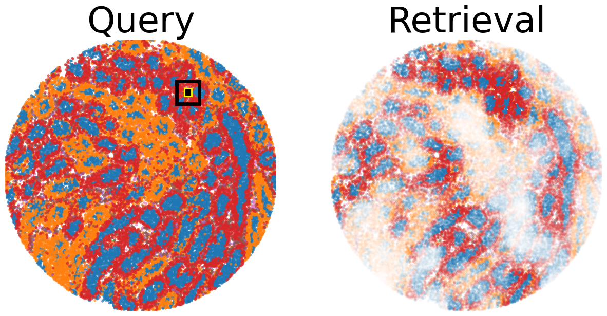
## Plot query patch and retrieval from  reference sample
# assign color to cell type
colors = sns.color_palette("tab10", 10).as_hex()
cdict = {
    'ES': colors[0],
    'RS': colors[1],
    'Myoid': colors[2],
    'SPC': colors[3],
    'SPG': colors[4],
    'Sertoli': colors[5],
    'Leydig': colors[6],
    'Endothelial': colors[7],
    'Macrophage': colors[8]
}

## Highlight query patch in query sample
highlight_list = [
    (3900., 1700., 'yellow')
]

# Create a figure
fig = plt.figure(figsize=(15,15))

# Plot Query
gs = gridspec.GridSpec(1, 2, hspace=0.0)
ax1 = fig.add_subplot(gs[0, 0])

scatter(adata_query, 'cell_type', x_key='y', y_key='x', mode='categorical', cdict=cdict, fig=fig, ax=ax1, ticks_off=True, show_legend=False, alpha=0.7, rasterized=True)
ax1.set_facecolor('white')
x_query, y_query, highlight_color = highlight_list[0]
patch_size = 128
rect = patches.Rectangle(
    (x_query - patch_size / 2, y_query - patch_size / 2),
    patch_size, patch_size,
    linewidth=2, edgecolor=highlight_color, facecolor='black')
ax1.add_patch(rect)

patch_size = 384
rect = patches.Rectangle(
    (x_query - patch_size / 2, y_query - patch_size / 2),
    patch_size, patch_size,
    linewidth=5, edgecolor='black', facecolor='none')
ax1.add_patch(rect)
ax1.set_title('Query', fontsize=50)

# Plot retrieval
ax2 = fig.add_subplot(gs[0, 1])
scatter(adata_ref_query, 'cell_type', alpha_key='sim', x_key='y', y_key='x', mode='categorical', cdict=cdict, ticks_off=True, fig=fig, ax=ax2, show_legend=False, linewidth=0, rasterized=True)
ax2.set_title('Retrieval', fontsize=50)
Text(0.5, 1.0, 'Retrieval')
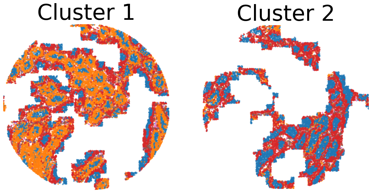
## Perform spatial clustering on the learned TissueMosaic representations

## Cluster the same adata sample we performed motif query on
adata_clustered = cluster(adata=adata_query,
                            key='dino',
                            n_neighbors=100,
                            leiden_res=[0.1, 0.2, 0.3])

## note that adata now has clustering annotations written in .obsm
adata_clustered
Running UMAP
Computing clusters
AnnData object with n_obs × n_vars = 35797 × 23706
    obs: 'x', 'y', 'UMI', 'cell_type', 'dino_spot_features_valid', 'train_test_fold_1', 'train_test_fold_2', 'train_test_fold_3', 'train_test_fold_4', 'sample_id', 'classify_condition', 'sim', 'leiden_feature_dino_res_0.1_one_hot', 'leiden_feature_dino_res_0.2_one_hot'
    uns: 'status'
    obsm: 'cell_type_proportions', 'dino', 'dino_spot_features', 'ncv_k10', 'ncv_k100', 'ncv_k25', 'leiden_feature_dino_res_0.3_one_hot'
## Plot clustering results

# Create a figure
fig = plt.figure(figsize=(15,15))
gs = gridspec.GridSpec(1, 2, hspace=0.0)

## plot cluster 1
ax1 = fig.add_subplot(gs[0, 0])
cluster_key = 'leiden_feature_dino_res_0.3_one_hot'

adata_cluster_1 = adata_clustered[adata_clustered.obsm[cluster_key][:,0] <= 0.999]

scatter(adata_cluster_1, 'cell_type', x_key='y', y_key='x', mode='categorical', cdict=cdict, ticks_off=True, show_legend=False, fig=fig, ax=ax1, alpha=0.7, rasterized=True)
ax1.set_title('Cluster 1', fontsize=50)

## plot cluster 2
ax2 = fig.add_subplot(gs[0, 1])

adata_cluster_2 = adata_clustered[adata_clustered.obsm[cluster_key][:,0] > 0.999]

scatter(adata_cluster_2, 'cell_type', x_key='y', y_key='x', mode='categorical', cdict=cdict, ticks_off=True, show_legend=False, fig=fig, ax=ax2, alpha=0.7, rasterized=True)
ax2.set_title('Cluster 2', fontsize=50)
Text(0.5, 1.0, 'Cluster 2')
Gene Regression
We can regress gene expression in elongated spermatid cells from the learned TissueMosaic representations by running the following commands in the console:
#set environment threads
export OMP_NUM_THREADS=1
export MKL_NUM_THREADS=1
export OPENBLAS_NUM_THREADS=1
export NUMEXPR_NUM_THREADS=1
# make output directory
mkdir ./tutorial/gr_results
python main_3_gene_regression.py\
    --anndata_in ./tutorial/testis_anndata_featurized\
    --out_dir ./tutorial/gr_results\
    --out_prefix dino_ctype\
    --feature_key dino_spot_features\
    --alpha_regularization_strength 0.01\
    --filter_feature 2.0\
    --fc_bc_min_umi 500\
    --fg_bc_min_pct_cells_by_counts 10\
    --cell_types ES
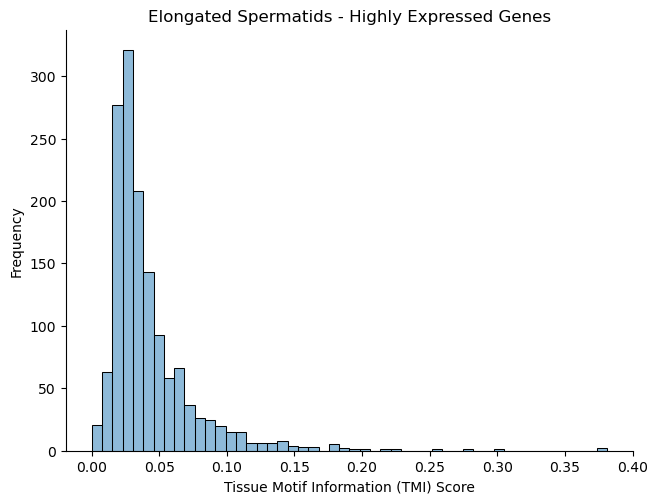
We can investigate the results
## Plot distribution of tissue motif information scores

cell_type_names = ["Elongated Spermatids"]

results_dir = './tutorial/gr_results'

ctype = "ES"

out_prefix = "dino_ctype"

rel_q_gk_outfile_name = out_prefix + '_' + ctype + f"_df_rel_q_gk_ssl.pickle"
rel_q_gk_outfile = os.path.join(results_dir, rel_q_gk_outfile_name)
rel_q_gk = pickle.load(open(rel_q_gk_outfile, 'rb'))

## flip sign of TMI score
rel_q_gk = -1 * rel_q_gk

## discard genes with TMI score < 0 (these are outlier genes whose performance is worse than baseline)
rel_q_gk = rel_q_gk[rel_q_gk > 0].dropna()

fig, ax = plt.subplots()
plt.tight_layout()
sns.histplot(rel_q_gk, bins=50, legend=False)
plt.ylabel('Frequency')
plt.xlabel('Tissue Motif Information (TMI) Score')
ax.tick_params(axis='y')
ax.tick_params(axis='x')
ax.spines['top'].set_visible(False)
ax.spines['right'].set_visible(False)
ax.spines['bottom']
ax.spines['left']
ax.set_title('Elongated Spermatids - Highly Expressed Genes')
Text(0.5, 1.0, 'Elongated Spermatids - Highly Expressed Genes')
rel_q_gk.sort_values(by=0).tail(n=10)
| 0 | |
|---|---|
| Tex33 | 0.184594 |
| Ccer1 | 0.192707 |
| Rnf151 | 0.199231 |
| 4933411K16Rik | 0.217950 |
| Smcp | 0.223001 |
| Fam71b | 0.251620 |
| Prm1 | 0.278291 |
| Prm2 | 0.302034 |
| Tnp2 | 0.376735 |
| Tnp1 | 0.381183 |
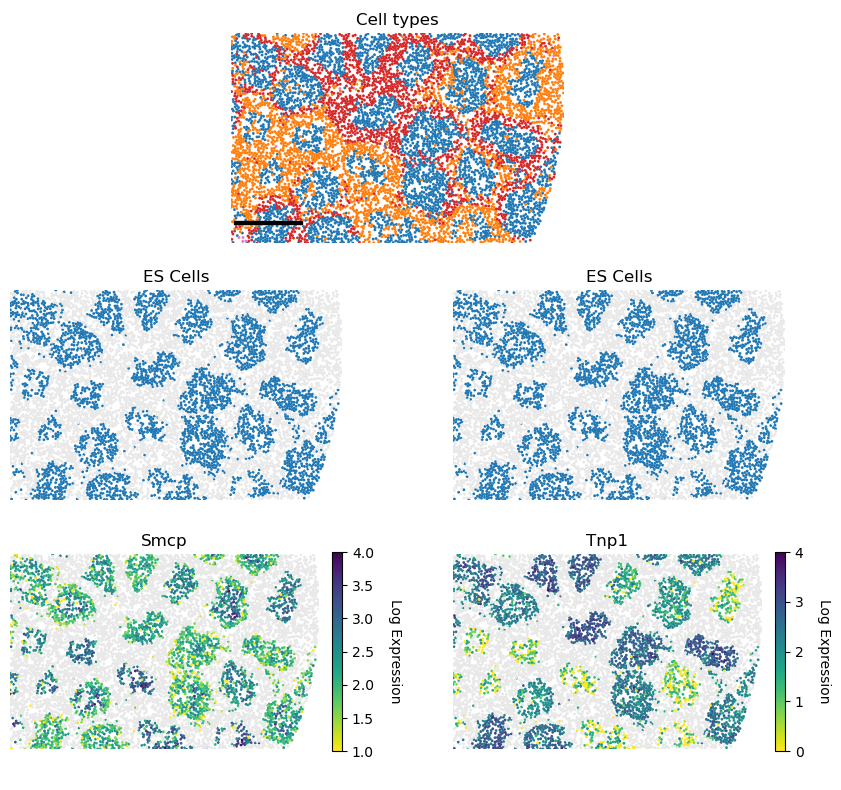
## Plot genes with high tissue motif information score back in space

## parameters
s = 5

i = np.where(np.array(fname_list) == 'wt2_dm_featurized.h5ad')[0][0] #3 ## wt 2
adata = anndata_list[i].copy()

## process gex
adata.obs['cell_type'] = adata.obsm['cell_type_proportions'].idxmax(axis=1)
sc.pp.normalize_total(adata)
sc.pp.log1p(adata)

kfold = 1

adata_kfold = adata[adata.obs[f'train_test_fold_{kfold}'] == 1]
adata_kfold_es = adata_kfold[adata_kfold.obs['cell_type'] == 'ES']
adata_kfold_nones = adata_kfold[adata_kfold.obs['cell_type'] != 'ES']

fig, axs = plt.subplots(figsize=(10,10))
axs.axis('off')

# Define the grid layout

gs = gridspec.GridSpec(3, 4, wspace=1.0, hspace=0.0) #, hspace=-0.1)


ax1 = fig.add_subplot(gs[0, 1:3])
# ax1.set_title('Testis', fontsize=labelfontsize, pad=labelpad)
scatter(adata_kfold, 'cell_type', x_key='x', y_key='y', mode='categorical', fig=fig, ax=ax1, cdict=cdict, s=s, ticks_off=True, show_legend=False,rasterized=True)
ax1.set_aspect('equal', 'box')
ax1.axis('off')
scalebar = AnchoredSizeBar(ax1.transData,
                           461.54, '', 'lower left',
                           pad=0.1,
                           color='black',
                           frameon=False,
                           size_vertical=20)
ax1.add_artist(scalebar)
ax1.set_title('Cell types')

prop_cycle = plt.rcParams['axes.prop_cycle']
colors = prop_cycle.by_key()['color']

# assign color to cell type
grey_hex = '#E8E8E8'
cdict_temp = {
    'ES': colors[0],
    'RS': grey_hex,
    'Myoid': grey_hex,
    'SPC': grey_hex,
    'SPG': grey_hex,
    'Sertoli': grey_hex,
    'Leydig': grey_hex,
    'Endothelial': grey_hex,
    'Macrophage': grey_hex
}

ax1 = fig.add_subplot(gs[1, :2])
scatter(adata_kfold, 'cell_type', x_key='x', y_key='y', mode='categorical', fig=fig, ax=ax1, cdict=cdict_temp, s=s, ticks_off=True, show_legend=False,rasterized=True)
ax1.set_aspect('equal', 'box')
ax1.axis('off')
ax1.set_title('ES Cells')

ax1 = fig.add_subplot(gs[1, 2:])
scatter(adata_kfold, 'cell_type', x_key='x', y_key='y', mode='categorical', fig=fig, ax=ax1, cdict=cdict_temp, s=s, ticks_off=True, show_legend=False,rasterized=True)
ax1.set_aspect('equal', 'box')
ax1.axis('off')
ax1.set_title('ES Cells')

# Second row, first plot
ax2 = fig.add_subplot(gs[2, :2])

gene = 'Smcp'

x_coord = adata_kfold_es.obs['x']
y_coord = adata_kfold_es.obs['y']
UMI = adata_kfold_es.obs['UMI']

gene_adata = adata_kfold_es[:,gene]
genex = np.squeeze(np.array(gene_adata.X.todense().flatten()))

ax2_sc = ax2.scatter(x_coord, y_coord, c=genex, s = s, marker='h', edgecolors='none', vmin=1, vmax=4, cmap='viridis_r',rasterized=True)
ax2.set_aspect('equal', 'box')
ax2.set_xlim((np.min(adata_kfold.obs['x'].values), np.max(adata_kfold.obs['x'].values)))
ax2.set_ylim((np.min(adata_kfold.obs['y'].values), np.max(adata_kfold.obs['y'].values)))
ax2.axes.invert_yaxis()
ax2.set_xticks([])
ax2.set_yticks([])

scatter(adata_kfold_nones, 'cell_type', x_key='x', y_key='y', mode='categorical', fig=fig, ax=ax2, cdict=cdict_temp, s=s, ticks_off=True, show_legend=False,rasterized=True)

ax2.set_title(gene)
ax2.spines['top'].set_visible(False)
ax2.spines['right'].set_visible(False)
ax2.spines['bottom'].set_visible(False)
ax2.spines['left'].set_visible(False)
ax2.set_ylabel('Log Expression')
ax2.axis('off')
cbar = plt.colorbar(ax2_sc, ax=ax2, label=None, fraction=0.030, pad=0.04)
cbar.set_label('Log Expression', rotation=270,labelpad=20)
cbar.ax.tick_params()


gene = 'Tnp1'

kfold = 1

adata_kfold = adata[adata.obs[f'train_test_fold_{kfold}'] == 1]
adata_kfold_es = adata_kfold[adata_kfold.obs['cell_type'] == 'ES']
adata_kfold_nones = adata_kfold[adata_kfold.obs['cell_type'] != 'ES']

x_coord = adata_kfold_es.obs['x']
y_coord = adata_kfold_es.obs['y']
UMI = adata_kfold_es.obs['UMI']

gene_adata = adata_kfold_es[:,gene]
genex = np.squeeze(np.array(gene_adata.X.todense().flatten()))

ax3 = fig.add_subplot(gs[2, 2:])


ax3_sc = ax3.scatter(x_coord, y_coord, c=genex, s = s, marker='h', edgecolors='none', vmin=0, vmax=4, cmap='viridis_r',rasterized=True)
ax3.set_aspect('equal', 'box')
ax3.set_xlim((np.min(adata_kfold.obs['x'].values), np.max(adata_kfold.obs['x'].values)))
ax3.set_ylim((np.min(adata_kfold.obs['y'].values), np.max(adata_kfold.obs['y'].values)))
ax3.axes.invert_yaxis()
ax3.set_xticks([])
ax3.set_yticks([])

scatter(adata_kfold_nones, 'cell_type', x_key='x', y_key='y', mode='categorical', fig=fig, ax=ax3, cdict=cdict_temp, s=s, ticks_off=True, show_legend=False,rasterized=True)


ax3.set_title(gene)
ax3.spines['top'].set_visible(False)
ax3.spines['right'].set_visible(False)
ax3.spines['bottom'].set_visible(False)
ax3.spines['left'].set_visible(False)
ax3.axis('off')
cbar = plt.colorbar(ax3_sc, ax=ax3, label=None, fraction=0.030, pad=0.04)
cbar.set_label('Log Expression', rotation=270,labelpad=20)
# cbar.ax.set_yticklabels([0.0, 2.0, 4.0])
Conditional Motif Enrichment
## perform conditional motif enrichment

## Run enrichment on motifs (with all cell types)

warnings.filterwarnings('ignore')

adata_enriched = conditional_motif_enrichment(adata_merged, feature_key="dino_spot_features",
                                              classify_or_regress="classify", alpha_regularization = [1000.0, 2500.0, 5000.0])

## can subset anndata to specific cell types to do enrichment in a cell-type specific manner
## ex: adata_es_merged = adata_merged[adata_merged.obs['cell_type'] == 'ES']
Running kfold 1
Running kfold 2
Running kfold 3
Running kfold 4
## write motif enriched anndatas to file

anndata_enriched_db = adata_enriched[adata_enriched.obs['predicted_condition'] >= 0]
anndata_enriched_db.write_h5ad('./tutorial/testis_anndata_enriched_db.h5ad')

anndata_enriched_wt = adata_enriched[adata_enriched.obs['predicted_condition'] < 0]
anndata_enriched_wt.write_h5ad('./tutorial/testis_anndata_enriched_wt.h5ad')
Run GEX regression on enriched anndatas
python main_3_gene_regression.py\
    --anndata_in ./tutorial/testis_anndata_enriched_wt.h5ad\
    --out_dir ./tutorial/gr_results\
    --out_prefix dino_enriched_wt_ctype\
    --feature_key dino_spot_features\
    --alpha_regularization_strength 0.01\
    --filter_feature 2.0\
    --fc_bc_min_umi=500\
    --fg_bc_min_pct_cells_by_counts 10\
    --cell_types ES


python main_3_gene_regression.py\
    --anndata_in ./tutorial/testis_anndata_enriched_db.h5ad\
    --out_dir ./tutorial/gr_results\
    --out_prefix dino_enriched_db_ctype\
    --feature_key dino_spot_features\
    --alpha_regularization_strength 0.01\
    --filter_feature 2.0\
    --fc_bc_min_umi=500\
    --fg_bc_min_pct_cells_by_counts 10\
    --cell_types ES
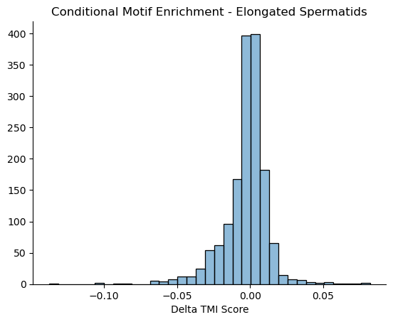
## look at delta TMI genes b/w enriched motifs

ctype = "ES"

out_dir = "./tutorial/gr_results"

wt_rel_q_gk_outfile_name = 'dino_enriched_wt_ctype' + '_' + ctype + f"_df_rel_q_gk_ssl.pickle"
wt_rel_q_gk_outfile = os.path.join(out_dir, wt_rel_q_gk_outfile_name)
wt_rel_q_gk = pickle.load(open(wt_rel_q_gk_outfile, 'rb'))
wt_rel_q_gk = -1 * wt_rel_q_gk
wt_rel_q_gk = wt_rel_q_gk[wt_rel_q_gk > 0]

db_rel_q_gk_outfile_name = 'dino_enriched_db_ctype' + '_' + ctype + f"_df_rel_q_gk_ssl.pickle"
db_rel_q_gk_outfile = os.path.join(out_dir, db_rel_q_gk_outfile_name)
db_rel_q_gk = pickle.load(open(db_rel_q_gk_outfile, 'rb'))
db_rel_q_gk = -1 * db_rel_q_gk
db_rel_q_gk = db_rel_q_gk[db_rel_q_gk > 0]


higher_si_in_db = db_rel_q_gk.sub(wt_rel_q_gk, fill_value=0).dropna()

print('Delta TMI < 0')
print(higher_si_in_db.sort_values(by=0).head(n=10))
print('Delta TMI > 0')
print(higher_si_in_db.sort_values(by=0).tail(n=10))

ax = sns.histplot(higher_si_in_db,bins=35, legend=False)
plt.ylabel('')
ax.tick_params(axis='both')  # Adjust labelsize as needed
ax.spines['top'].set_visible(False)
ax.spines['right'].set_visible(False)
ax.set_title('Conditional Motif Enrichment - Elongated Spermatids')
ax.set_xlabel('Delta TMI Score')
Delta TMI < 0
                      0
Lars2         -0.137719
Camk1d        -0.104417
Prss51        -0.100615
Cmss1         -0.091653
Pde1c         -0.085228
Rasa3         -0.065679
Grin2b        -0.063508
Nat9          -0.063372
Noxred1       -0.063292
1700125H03Rik -0.063064
Delta TMI > 0
                      0
mt-Rnr2        0.046020
Spata18        0.047754
Gapdhs         0.052634
Gsg1           0.053069
Hmgb4          0.055628
Odf1           0.058060
Odf2           0.065754
1700001P01Rik  0.071021
Tnp1           0.078064
Tnp2           0.082039
Text(0.5, 0, 'Delta TMI Score')
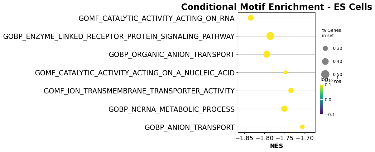
## gene set enrichment analysis on delta TMI scores

pre_res = gp.prerank(rnk=higher_si_in_db, # or rnk = rnk,
                     gene_sets='/home/skambha6/chenlab/utils/m5.go.v2022.1.Mm.symbols.gmt', ## replace with path to your gene set
                     threads=4,
                     min_size=10,
                     max_size=1000,
                     permutation_num=10000, # reduce number to speed up testing
                     outdir=None, # don't write to disk
                     seed=6,
                     verbose=True, # see what's going on behind the scenes
                    )

pre_res.res2d.sort_values(by='FDR q-val', ascending = True, inplace=True)
# print(pre_res.res2d.head(15)[['Term', 'NES', 'NOM p-val', 'FDR q-val', 'Lead_genes']])

ax = gp.dotplot(pre_res.res2d,
             column="FDR q-val",
             title='Conditional Motif Enrichment - ES Cells',
             cmap=plt.cm.viridis,
             size=6, # adjust dot size
             figsize=(4,5), thresh=0.25, cutoff=0.25, show_ring=False)
2024-06-25 19:26:19,934 [INFO] Parsing data files for GSEA.............................
2024-06-25 19:26:20,111 [INFO] 9435 gene_sets have been filtered out when max_size=1000 and min_size=10
2024-06-25 19:26:20,112 [INFO] 1125 gene_sets used for further statistical testing.....
2024-06-25 19:26:20,112 [INFO] Start to run GSEA...Might take a while..................
2024-06-25 19:26:40,262 [INFO] Congratulations. GSEApy runs successfully................